Linear Regression Fundamentals Problem Set
Instructions
This problem set covers the fundamental concepts of linear regression, including matrix formulations, geometric interpretations, and computational methods. Show all work and provide clear explanations for your reasoning.
Problem 1
Consider the following dataset with two predictors:
| Observation | x1 | x2 | y |
|---|---|---|---|
| 1 | 2 | 1 | 5.2 |
| 2 | 3 | 4 | 8.1 |
| 3 | 1 | 2 | 4.8 |
| 4 | 4 | 3 | 9.5 |
a) Write out the design matrix X for the multiple regression model with intercept term.
b) Calculate \(\mathbf{X}^T\mathbf{X}\) and \(\mathbf{X}^T\mathbf{y}\) by hand. Show your matrix multiplication steps.
c) Using your results from Part B, set up the normal equations \(\mathbf{X}^T\mathbf{X}\hat\beta=\mathbf{X}^T\mathbf{y}\) and solve for the coefficient vector \(\hat\beta\). (You can use R if you need to take an inverse).
d) Verify your answer using R’s built-in functions.
Problem 2
Using the data from Problem 1 and your estimated coefficients:
a) Calculate the predicted values \(\hat{y}_i\) for each observation by hand.
b) Calculate the residuals \(\hat\varepsilon=y_i-\hat{y}_i\) for each observation.
c) Compute the sum of squared errors (SSE) using both formulations:
- Individual terms: SSE \(= \sum(y_i - \hat{y}_i)^2\)
- Matrix form: SSE \(= (\mathbf{y}-\mathbf{X}\hat\beta)^T(\mathbf{y}-\mathbf{X}\hat\beta)\)
d) Verify that your residuals sum to approximately zero and explain why this should be true geometrically.
Problem 3
a) For simple linear regression with n = 3 observations and design matrix:
\[\mathbf{X} = \begin{bmatrix}1 & 2\\1 & 4\\1&6\end{bmatrix}\]
Calculate the hat matrix (\(\mathbf{H}\)) by hand (you can use R if you need to take an inverse).
b) Verify that \(\mathbf{H}\) is idempotent.
c) Show that \(\mathbf{H}\) is symmetric and interpret what this property means geometrically.
Problem 4
Consider the simple linear regression case with the design matrix from Problem 3.
a) Write out two specific vectors that lie in the column space of \(\mathbf{X}\). Explain what these vectors represent in terms of the regression model.
b) If the observed response vector is \(\mathbf{y} = \begin{bmatrix}3\\7\\12\end{bmatrix}\), explain why this vector likely does NOT lie exactly in the column space of \(\mathbf{X}\). What does this mean practically?
c) Calculate the projection of \(\mathbf{y}\) onto the column space (i.e., \(\mathbf{\hat{y}} = \mathbf{Hy}\)) and show that the residual vector is orthogonal to the column space by verifying \(\mathbf{X}^T\hat\varepsilon=0\).
Problem 5
a) Starting from the geometric principle that residuals must be orthogonal to the column space of \(\mathbf{X}\), derive the normal equations step by step. Begin with the condition \(\mathbf{X}^T\hat\varepsilon = 0\) and show all algebraic steps to arrive at \(\mathbf{X}^T\mathbf{X}\hat\beta=\mathbf{X}^T\mathbf{y}\).
b) Explain why we multiply both sides by \((\mathbf{X}^T\mathbf{X})^{-1}\) to solve for \(\hat\beta\), and under what conditions this inverse might not exist.
c) Show that the least squares estimator \(\hat\beta = (\mathbf{X}^T\mathbf{X})^{-1}\mathbf{X}^T\mathbf{y}\) minimizes the sum of squared errors by demonstrating that this solution satisfies the orthogonality condition.
Problem 6
You are given the following dataset with 10 observations:
| x | y |
|---|---|
| 1 | 4.8 |
| 2 | 6.2 |
| 3 | 8.1 |
| 4 | 9.9 |
| 5 | 11.5 |
| 6 | 13.8 |
| 7 | 15.2 |
| 8 | 17.1 |
| 9 | 18.9 |
| 10 | 21.3 |
a) Implement the least squares solution in R using matrix operations. Calculate \(\hat\beta\) without using lm().
b) Compare your results with R’s lm() function and verify they match.
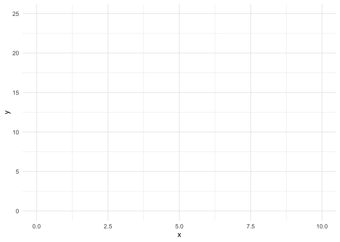
c) Using the grid below, hand-draw the following elements:
- Plot the 10 data points from the table above
- Draw the true regression line: y = 3.5 + 1.8x (shown as a dashed line)
- Draw your fitted regression line from Part A (shown as a solid line)
- Label both lines clearly in your plot
(You don’t have to upload this drawing on Canvas, but make sure you do it and understand it, we will do it during the board work portion in class.)
d) Based on your plot, comment on how well the fitted line approximates the true relationship. What does this tell you about the effectiveness of least squares estimation?