Exercise 1

Exercise 1: Login to RStudio Pro

1. Go to course website → Computing → Using the RStudio Server
2. Follow login instructions
3. Log in with your credentials

Check: You should see the RStudio interface with 4 panes.

---

Exercise 2: Create RStudio Project

1. File → New Project → New Directory → New Project
2. Name: ex-1
3. Click Create Project

Check: Project name appears in top-right corner.

---

Exercise 3: Create Quarto Document

1. File → New File → Quarto Document
2. Title: “My First Analysis”
3. Save as analysis.qmd

Check: New .qmd file is open and saved.

---

Exercise 4: Install faraway Package and Load Data

Run this code in the console ONCE:

install.packages("faraway")

Then run this:

library(faraway)
library(ggplot2)

# Test it works
data(teengamb)
head(teengamb)

  sex status income verbal gamble
1   1     51   2.00      8    0.0
2   1     28   2.50      8    0.0
3   1     37   2.00      6    0.0
4   1     28   7.00      4    7.3
5   1     65   2.00      8   19.6
6   1     61   3.47      6    0.1

Check: You see the teengamb dataset.

Now run this in the console:

?teengamb

Question: What is in this dataset?

Action: Add the code below to your .qmd file along with a short description of the data.

library(faraway)
library(ggplot2)
data(teengamb)

---

Exercise 5: Linear Model and Plot

Add the following code to your .qmd file. Try running it.

# Fit linear model
model1 <- lm(gamble ~ income, data = teengamb)
summary(model1)

Call:
lm(formula = gamble ~ income, data = teengamb)

Residuals:
    Min      1Q  Median      3Q     Max 
-46.020 -11.874  -3.757  11.934 107.120 

Coefficients:
            Estimate Std. Error t value Pr(>|t|)    
(Intercept)   -6.325      6.030  -1.049      0.3    
income         5.520      1.036   5.330 3.05e-06 ***
---
Signif. codes:  0 '***' 0.001 '**' 0.01 '*' 0.05 '.' 0.1 ' ' 1

Residual standard error: 24.95 on 45 degrees of freedom
Multiple R-squared:  0.387, Adjusted R-squared:  0.3734 
F-statistic: 28.41 on 1 and 45 DF,  p-value: 3.045e-06

# Create plot
ggplot(teengamb, aes(x = income, y = gamble)) +
  geom_point() +
  geom_smooth(method = "lm", formula = "y ~ x") +
  labs(title = "Income vs Gambling",
       x = "Income", 
       y = "Gambling")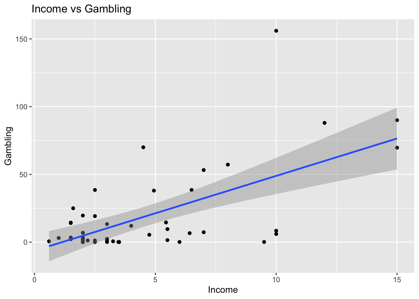

Check: You have model output and a scatter plot with trend line.

---

Finish

Click “Render” to create your HTML report. Upload your .html file in Canvas under Exercise 1